Drift Detection with datadriftR

Introduction

In production, the data generating process rarely stays still. Seasonality, product changes, user behavior, and policy updates can shift the distribution of your features—and sometimes even change the relationship between features and the target.

Example (concept drift): You train a model to predict whether electricity prices will go up based on demand and price signals. After a market reform, the same demand level can imply a different price movement. In practice this often shows up as a rising error rate or shifting model outputs.

datadriftR helps you detect these shifts early in streaming settings, so you can trigger investigation, retraining, or alerts.

Drift Taxonomy

Many “drift” problems are forms of dataset shift:

\[P_{train}(X, Y) \neq P_{prod}(X, Y)\]

What changed?

• Covariate shift: \(P(X)\) changes while \(P(Y|X)\) stays roughly the same.
• Concept drift: \(P(Y|X)\) changes (the mapping from inputs to outputs changes).

Drift Patterns

Drift can also differ by how it unfolds over time:

• Abrupt: change happens at once (deployments, outages, policy changes)
• Gradual: mixture of old/new concepts (slow adoption, rollout)
• Incremental: continuously moving distribution (wear-and-tear, trend)
• Recurring: seasonal or cyclical patterns (day/night, weekdays, holidays)

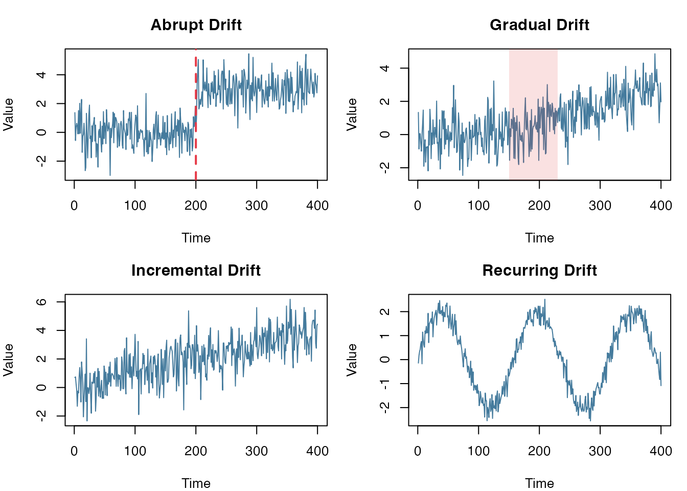
Common drift patterns

Available Methods

Method	What you feed
DDM, EDDM, HDDM-A/W	Binary (0/1) error stream
KSWIN, ADWIN, Page-Hinkley, KL Divergence	Numeric stream (or rolling window/batches)
ProfileDifference	Two profiles (e.g., PDPs)

---

Quick Start

Quick start with detect_drift():

set.seed(1)
x <- c(rnorm(300, 0, 1), rnorm(200, 3, 1))

detect_drift(x, method = "page_hinkley", delta = 0.05, threshold = 50)
#>   index    value  type
#> 1   315 2.964078 drift

---

Part 1: Error-Rate Detectors (Binary Stream)

These methods monitor a stream of prediction errors:

error_stream <- as.integer(y_pred != y_true)

They work well when you can observe labels reasonably quickly (or with a known delay).

Simulating Model Errors

set.seed(123)

n_good <- 500
n_bad <- 500
error_stream <- c(
  rbinom(n_good, 1, prob = 0.05),
  rbinom(n_bad, 1, prob = 0.30)
)
true_drift_error <- n_good + 1

Comparing All Error-Rate Methods

error_methods <- c("ddm", "eddm", "hddm_a", "hddm_w")

first_index <- function(res, type) {
  idx <- res$index[res$type == type]
  if (length(idx) == 0) NA_integer_ else idx[1]
}

error_results <- do.call(rbind, lapply(error_methods, function(m) {
  res <- detect_drift(error_stream, method = m, include_warnings = TRUE)
  warning_idx <- first_index(res, "warning")
  drift_idx <- first_index(res, "drift")
  data.frame(
    Method = gsub("_", "-", toupper(m)),
    Warning = warning_idx,
    Drift = drift_idx,
    DriftDelay = if (!is.na(drift_idx)) drift_idx - true_drift_error else NA,
    stringsAsFactors = FALSE
  )
}))

error_results
#>   Method Warning Drift DriftDelay
#> 1    DDM     401   538         37
#> 2   EDDM      NA   461        -40
#> 3 HDDM-A     548   570         69
#> 4 HDDM-W     546   549         48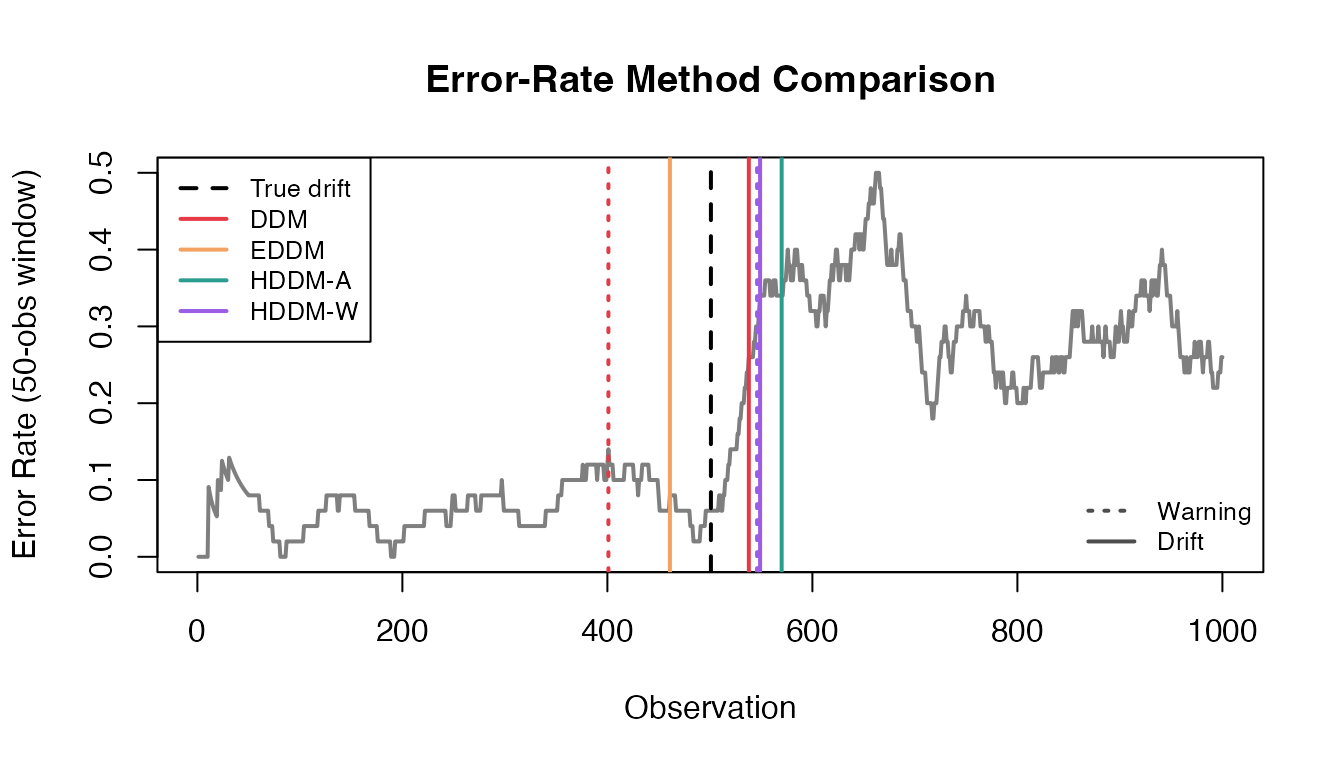

Online Processing (Streaming)

ddm <- DDM$new()
drifts <- c()

for (i in seq_along(error_stream)) {
  ddm$add_element(error_stream[i])
  if (ddm$change_detected) {
    drifts <- c(drifts, i)
    ddm$reset()
  }
}

data.frame(Method = "DDM", True = true_drift_error, Detected = drifts)
#>   Method True Detected
#> 1    DDM  501      538

The loop above is the “low-level” way to run a detector. For convenience, detect_drift() provides the same idea as a single function call:

ddm_res <- detect_drift(error_stream, method = "ddm", include_warnings = FALSE)
ddm_res
#>   index value  type
#> 1   538     1 drift

---

Part 2: Continuous-Stream Detectors (Numeric Data)

These methods work with any numeric stream—sensor readings, feature values, model predictions.

Simulating Sensor Data

set.seed(456)

n_normal <- 300
n_faulty <- 200
sensor_stream <- c(
  rnorm(n_normal, mean = 20, sd = 1),
  rnorm(n_faulty, mean = 28, sd = 2)
)
true_drift_sensor <- n_normal + 1

Comparing All Distribution Methods

dist_methods <- c("kswin", "adwin", "page_hinkley")

dist_results <- do.call(rbind, lapply(dist_methods, function(m) {
  res <- detect_drift(sensor_stream, method = m)
  data.frame(
    Method = gsub("_", "-", toupper(m)),
    Detected = if (nrow(res) > 0) res$index[1] else NA,
    Delay = if (nrow(res) > 0) res$index[1] - true_drift_sensor else NA,
    stringsAsFactors = FALSE
  )
}))

dist_results
#>         Method Detected Delay
#> 1        KSWIN      313    12
#> 2        ADWIN      320    19
#> 3 PAGE-HINKLEY      306     5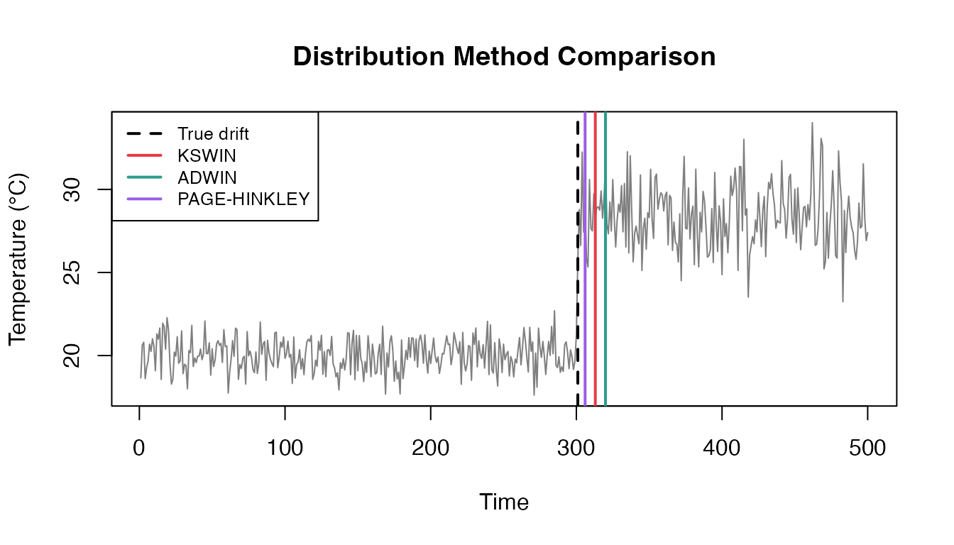

---

Part 3: KL Divergence

Sometimes you want to compare recent values to a reference window (latency, transaction amount, sensor readings, model scores).

KLDivergence is a simple histogram-based implementation of Kullback–Leibler divergence. When the divergence crosses a threshold, it flags drift.

set.seed(789)

n_ref <- 400
n_shift <- 400
latency_ms <- c(
  rlnorm(n_ref, meanlog = log(100), sdlog = 0.25),
  rlnorm(n_shift, meanlog = log(180), sdlog = 0.30)
)
true_drift_kld <- n_ref + 1

window <- 200
kld <- KLDivergence$new(bins = 30, drift_level = 0.15)
kld$set_initial_distribution(latency_ms[1:window])

kl <- rep(NA_real_, length(latency_ms))
for (t in (window + 1):length(latency_ms)) {
  current <- latency_ms[(t - window + 1):t]
  kld$add_distribution(current)
  kl[t] <- kld$get_kl_result()
}

detected_kld <- which(kl > kld$drift_level)[1]
data.frame(True = true_drift_kld, Detected = detected_kld, Threshold = kld$drift_level)
#>   True Detected Threshold
#> 1  401      295      0.15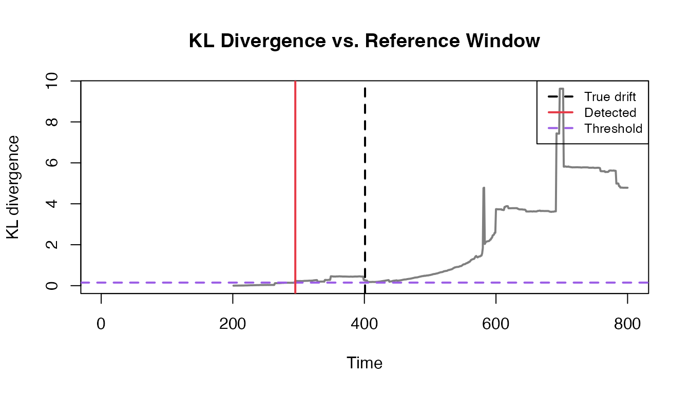

---

Part 4: ProfileDifference (Model Behavior)

Partial Dependence Profiles (PDPs) show how a model’s prediction changes with a feature. When concept drift occurs, the relationship between features and target changes—PDPs capture this.

Available Methods

Method	Description
pdi	Profile Disparity Index - compares derivative signs
L2	L2 norm between profiles
L2_derivative	L2 norm of profile derivatives

Example: Electricity Prices (elec2)

The elec2 dataset from the dynaTree package is a classic benchmark for concept drift—Australian electricity prices where market dynamics changed over time. This section requires the optional packages dynaTree and ranger. For readability we rename x1..x4/y, and for speed we train on a small subset from each time period.

library(dynaTree)
library(ranger)

elec2_env <- new.env(parent = emptyenv())
data("elec2", package = "dynaTree", envir = elec2_env)
elec2_df <- get("elec2", envir = elec2_env)
stopifnot(is.data.frame(elec2_df))

names(elec2_df) <- c("nswprice", "nswdemand", "vicprice", "vicdemand", "class_raw")
elec2_df$class <- factor(elec2_df$class_raw, levels = c(1, 2), labels = c("DOWN", "UP"))
elec2_df$class_raw <- NULL

split_idx <- floor(nrow(elec2_df) / 2)
period1_data <- elec2_df[1:split_idx, ]
period2_data <- elec2_df[(split_idx + 1):nrow(elec2_df), ]

n_train <- min(2000, nrow(period1_data), nrow(period2_data))
period1_train <- period1_data[1:n_train, ]
period2_train <- period2_data[1:n_train, ]

rf1 <- ranger(class ~ nswprice + nswdemand + vicprice + vicdemand,
                 data = period1_train, probability = TRUE, num.trees = 200, seed = 1)
rf2 <- ranger(class ~ nswprice + nswdemand + vicprice + vicdemand,
                 data = period2_train, probability = TRUE, num.trees = 200, seed = 1)

compute_pdp_rf <- function(model, data, var, grid) {
  preds <- sapply(grid, function(val) {
    newdata <- data
    newdata[[var]] <- val
    mean(predict(model, newdata)$predictions[, "UP"])
  })
  list(x = grid, y = preds)
}

demand_grid <- seq(min(elec2_df$nswdemand), max(elec2_df$nswdemand), length.out = 50)
pdp1 <- compute_pdp_rf(rf1, period1_train, "nswdemand", demand_grid)
pdp2 <- compute_pdp_rf(rf2, period2_train, "nswdemand", demand_grid)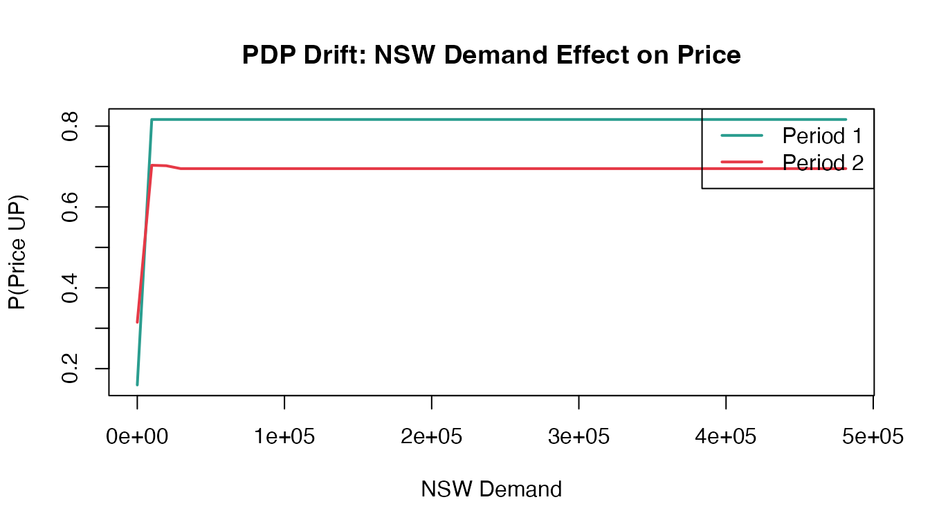

Comparing All Methods

# PDI (Profile Disparity Index)
pd_pdi <- ProfileDifference$new(method = "pdi", deriv = "gold")
pd_pdi$set_profiles(pdp1, pdp2)
res_pdi <- pd_pdi$calculate_difference()

# L2 norm
pd_l2 <- ProfileDifference$new(method = "L2")
pd_l2$set_profiles(pdp1, pdp2)
res_l2 <- pd_l2$calculate_difference()

# L2 derivative
pd_l2d <- ProfileDifference$new(method = "L2_derivative")
pd_l2d$set_profiles(pdp1, pdp2)
res_l2d <- pd_l2d$calculate_difference()

data.frame(
  Method = c("PDI", "L2", "L2_derivative"),
  Distance = round(c(res_pdi$distance, res_l2$distance, res_l2d$distance), 4)
)
#>          Method Distance
#> 1           PDI   0.0284
#> 2            L2  84.4088
#> 3 L2_derivative   0.0005

Higher distance indicates the model learned different demand-price relationships in each period—concept drift detected.

---

Quick Reference

What you monitor	Typical signal	Recommended
Binary error stream	Sudden or gradual accuracy drop	DDM, EDDM, HDDM-A/W
Numeric stream	Feature/sensor/score distribution shift	KSWIN, ADWIN, Page-Hinkley
Reference vs. current batch	Periodic samples (e.g., daily latency)	KLDivergence
Model behavior profiles	PDP/feature effect changes	ProfileDifference

---

References

The drift detection methods implemented in datadriftR are based on established algorithms from the streaming machine learning literature. For Python implementations, see:

• River (riverml.xyz): Online machine learning library with drift detectors
• scikit-multiflow (scikit-multiflow.github.io): Stream learning framework

Source code: github.com/ugurdar/datadriftR